self.w = np.linalg.inv(X_.T@X_)@X_.T@yLinear Regression
Implementing linear regression in two ways
1. Analytical formula for \(\hat{w}\)
The first way to implement linear regression is by using the analytical formula that gives us the \(\hat{w}\) to minimize \(L(w)\):
2. Gradient descent
We could also use the regular gradient descent to compute \(\hat{w}\). To reduce time complexity, we precompute P = X_.T@X and q = X.T@y, and then pass them to gradient() in the for-loop where we update the gradient:
self.w -= 2*alpha*self.gradient(P, q, self.w)Experiments
Increasing the number of features
In this experiment, I explore how the training score and validation score change as the number of features increases.
from linear_regression import LinearRegression
from matplotlib import pyplot as plt
import numpy as np

# functions for data generation
def pad(X):
    return np.append(X, np.ones((X.shape[0], 1)), 1)

def LR_data(n_train = 100, n_val = 100, p_features = 1, noise = .1, w = None):
    if w is None:
        w = np.random.rand(p_features + 1) + .2

    X_train = np.random.rand(n_train, p_features)
    y_train = pad(X_train)@w + noise*np.random.randn(n_train)

    X_val = np.random.rand(n_val, p_features)
    y_val = pad(X_val)@w + noise*np.random.randn(n_val)

    return X_train, y_train, X_val, y_val
I increase the number of features used in the model from 1 to n_train-1 and plot the change in training and validation scores.
# generate data
n_train = 100
n_val = 100
noise = 0.2
train_scores = []
val_scores = []

# increase p_features from 1 to n_train-1 and calculate training and validation scores for each
for p_features in np.arange(1, n_train):
    # create data
    X_train, y_train, X_val, y_val = LR_data(n_train, n_val, p_features, noise)
    LR = LinearRegression()
    LR.fit(X_train, y_train)
    train_scores.append(LR.score(X_train, y_train))
    val_scores.append(LR.score(X_val, y_val))


# plot
plt.plot(np.arange(1, n_train), train_scores, label = "Training scores")

# plot
plt.plot(np.arange(1, n_train), val_scores, label = "Validation scores")

xlab = plt.xlabel("Number of features")
ylab = plt.ylabel("Score")
legend = plt.legend() 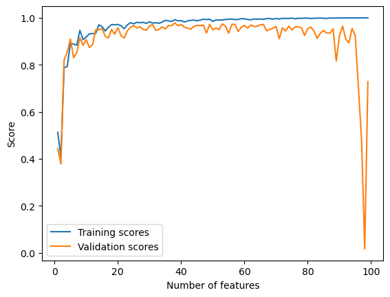
We can observe from the chart that the training score increased all the way to 1.0 as the number of features increases. The validation score, however, has been fluctuating and forms a slightly downward trend, and dramatically decreased to almost 0 when the number of features reached ~99.
This is a demonstration of overfitting. With too many features, the model becomes increasingly accurate in describing the trend in the training data, but at the same time takes into account more noise from the training data that doesn’t generate to the rest of the data. As a result, validation scores decrease.
LASSO regularization
To fix overfitting, I experiment with LASSO regularization:
from sklearn.linear_model import Lasso

# generate data
n_train = 100
n_val = 100
noise = 0.2
train_scores = []
val_scores = []

# increase p_features from 1 to n_train-1 and calculate training and validation scores for each
for p_features in np.arange(1, n_train + 10):
    # create data
    X_train, y_train, X_val, y_val = LR_data(n_train, n_val, p_features, noise)
    L = Lasso(alpha = 0.001)
    L.fit(X_train, y_train)
    train_scores.append(L.score(X_train, y_train))
    val_scores.append(L.score(X_val, y_val))


# plot
plt.plot(np.arange(1, n_train + 10), train_scores, label = "Training scores")
plt.plot(np.arange(1, n_train + 10), val_scores, label = "Validation scores")

xlab = plt.xlabel("Number of features")
ylab = plt.ylabel("Score")
legend = plt.legend() 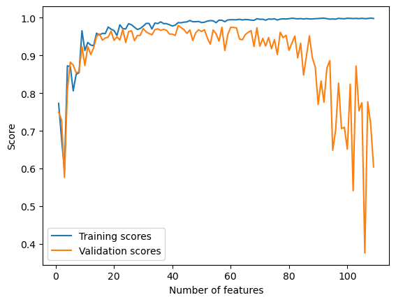
Using LASSO regularization, the validation scores still drops as the number of features increases, but there is no dramatical decrease as the number of features approaches, or even exceeds the number of data points. This is because LASSO is able to force entries of the weight vector to zero, which can help eliminate the effect of features that act as noise to the model.
Bikeshare data set
In this section, I train my linear regression model to a bikeshare data set.
# import data
import pandas as pd
from sklearn.model_selection import train_test_split
bikeshare = pd.read_csv("https://philchodrow.github.io/PIC16A/datasets/Bike-Sharing-Dataset/day.csv")

bikeshare.head()| instant | dteday | season | yr | mnth | holiday | weekday | workingday | weathersit | temp | atemp | hum | windspeed | casual | registered | cnt | |
|---|---|---|---|---|---|---|---|---|---|---|---|---|---|---|---|---|
| 0 | 1 | 2011-01-01 | 1 | 0 | 1 | 0 | 6 | 0 | 2 | 0.344167 | 0.363625 | 0.805833 | 0.160446 | 331 | 654 | 985 |
| 1 | 2 | 2011-01-02 | 1 | 0 | 1 | 0 | 0 | 0 | 2 | 0.363478 | 0.353739 | 0.696087 | 0.248539 | 131 | 670 | 801 |
| 2 | 3 | 2011-01-03 | 1 | 0 | 1 | 0 | 1 | 1 | 1 | 0.196364 | 0.189405 | 0.437273 | 0.248309 | 120 | 1229 | 1349 |
| 3 | 4 | 2011-01-04 | 1 | 0 | 1 | 0 | 2 | 1 | 1 | 0.200000 | 0.212122 | 0.590435 | 0.160296 | 108 | 1454 | 1562 |
| 4 | 5 | 2011-01-05 | 1 | 0 | 1 | 0 | 3 | 1 | 1 | 0.226957 | 0.229270 | 0.436957 | 0.186900 | 82 | 1518 | 1600 |
# plot the number of casual users over time
fig, ax = plt.subplots(1, figsize = (7, 3))
ax.plot(pd.to_datetime(bikeshare['dteday']), bikeshare['casual'])
ax.set(xlabel = "Day", ylabel = "# of casual users")
l = plt.tight_layout()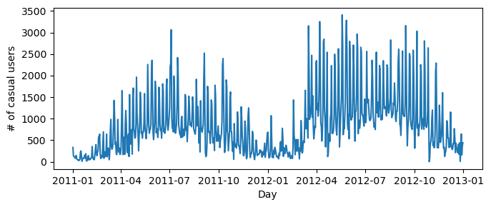
# transforming data
cols = ["casual",
        "mnth",
        "weathersit",
        "workingday",
        "yr",
        "temp",
        "hum",
        "windspeed",
        "holiday"]

bikeshare = bikeshare[cols]

bikeshare = pd.get_dummies(bikeshare, columns = ['mnth'], drop_first = "if_binary")
bikeshare| casual | weathersit | workingday | yr | temp | hum | windspeed | holiday | mnth_2 | mnth_3 | mnth_4 | mnth_5 | mnth_6 | mnth_7 | mnth_8 | mnth_9 | mnth_10 | mnth_11 | mnth_12 | |
|---|---|---|---|---|---|---|---|---|---|---|---|---|---|---|---|---|---|---|---|
| 0 | 331 | 2 | 0 | 0 | 0.344167 | 0.805833 | 0.160446 | 0 | 0 | 0 | 0 | 0 | 0 | 0 | 0 | 0 | 0 | 0 | 0 |
| 1 | 131 | 2 | 0 | 0 | 0.363478 | 0.696087 | 0.248539 | 0 | 0 | 0 | 0 | 0 | 0 | 0 | 0 | 0 | 0 | 0 | 0 |
| 2 | 120 | 1 | 1 | 0 | 0.196364 | 0.437273 | 0.248309 | 0 | 0 | 0 | 0 | 0 | 0 | 0 | 0 | 0 | 0 | 0 | 0 |
| 3 | 108 | 1 | 1 | 0 | 0.200000 | 0.590435 | 0.160296 | 0 | 0 | 0 | 0 | 0 | 0 | 0 | 0 | 0 | 0 | 0 | 0 |
| 4 | 82 | 1 | 1 | 0 | 0.226957 | 0.436957 | 0.186900 | 0 | 0 | 0 | 0 | 0 | 0 | 0 | 0 | 0 | 0 | 0 | 0 |
| ... | ... | ... | ... | ... | ... | ... | ... | ... | ... | ... | ... | ... | ... | ... | ... | ... | ... | ... | ... |
| 726 | 247 | 2 | 1 | 1 | 0.254167 | 0.652917 | 0.350133 | 0 | 0 | 0 | 0 | 0 | 0 | 0 | 0 | 0 | 0 | 0 | 1 |
| 727 | 644 | 2 | 1 | 1 | 0.253333 | 0.590000 | 0.155471 | 0 | 0 | 0 | 0 | 0 | 0 | 0 | 0 | 0 | 0 | 0 | 1 |
| 728 | 159 | 2 | 0 | 1 | 0.253333 | 0.752917 | 0.124383 | 0 | 0 | 0 | 0 | 0 | 0 | 0 | 0 | 0 | 0 | 0 | 1 |
| 729 | 364 | 1 | 0 | 1 | 0.255833 | 0.483333 | 0.350754 | 0 | 0 | 0 | 0 | 0 | 0 | 0 | 0 | 0 | 0 | 0 | 1 |
| 730 | 439 | 2 | 1 | 1 | 0.215833 | 0.577500 | 0.154846 | 0 | 0 | 0 | 0 | 0 | 0 | 0 | 0 | 0 | 0 | 0 | 1 |
731 rows × 19 columns
# train-test split
train, test = train_test_split(bikeshare, test_size = .2, shuffle = False)

X_train = train.drop(["casual"], axis = 1)
y_train = train["casual"]

X_test = test.drop(["casual"], axis = 1)
y_test = test["casual"]
# fit and score the model
LR = LinearRegression()
LR.fit(X_train, y_train)
LR.score(X_train, y_train)0.7318355359284503The model has a score of 0.73.
# compute predictions and visualize in comparison to actual test data
y_hat = LR.predict(X_test)

plt.plot(np.arange(len(y_hat)), y_hat, label = "Predictions")
plt.plot(np.arange(len(y_hat)), y_test, label = "Test data")

xlab = plt.xlabel("Day")
ylab = plt.ylabel("Number of casual users")
legend = plt.legend() 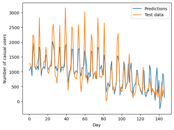
It seems that the model does a good job in predicting the general trend in the data – the overall decreasing number of users and the timing of peaks. However, it tends to underestimate the minimum and maximum values.
Finally, I will look into the weight vector and see what it reveals about people’s preference of when to use bikeshare.
# compare weight vector to list of features
feature_weights = pd.DataFrame(LR.w[:-1], X_train.columns)
feature_weights| 0 | |
|---|---|
| weathersit | -108.371136 |
| workingday | -791.690549 |
| yr | 280.586927 |
| temp | 1498.715113 |
| hum | -490.100340 |
| windspeed | -1242.800381 |
| holiday | -235.879349 |
| mnth_2 | -3.354397 |
| mnth_3 | 369.271956 |
| mnth_4 | 518.408753 |
| mnth_5 | 537.301886 |
| mnth_6 | 360.807998 |
| mnth_7 | 228.881481 |
| mnth_8 | 241.316412 |
| mnth_9 | 371.503854 |
| mnth_10 | 437.600848 |
| mnth_11 | 252.433004 |
| mnth_12 | 90.821460 |
We can observe a couple of interesting trends from the magnitude and direction of the weights: 1. People use bikeshare more when the weather is nicer – especially when it is warmer and there is less wind. It is also interesting, though, that the weathersit variable is slightly negatively correlated with the number of users. I wonder what exactly this variable is measuring. 2. People use bikeshare the most in April and May. This makes sense because weather is the best during this time of the year, while summer is too hot and winter is too cold. 3. People use bikeshare more on weekends but less on holidays.