Perceptron

Implementing the perceptron

I implemented the perceptron update with the following steps:

Modifying the feature matrix \(X\) and vector of labels \(y\). This includes appending a column of 1s to \(X\) and turning \(y\) into a vector of -1s and 1s.
Initializing a random weight vector \(w\).
In a for-loop that breaks either when accuracy reaches 1 or when the specified max_steps is reached,
1. Pick a random data point with index \(i\) and access its features \(x_{i}\) and label \(y_{i}\);
2. Compute the predicted label \(\hat{y}\) using the current \(w\);
3. Perform update if \(y\) * \(\hat{y}\) < 0:

self.w = self.w + (y_i*y_hat < 0) * (y_i * x_)

Where only when y_i * y_hat < 0 is (y_i * x_) added to the current w.

Finally, the accuracy of the current \(w\) is computed by using \(w\) to predict labels for all data points, and then calculating the number of correct predictions compared to \(y\). This accuracy is then appended to the history array.

Experiments

Linearly separable 2D data

from perceptron import Perceptron
import numpy as np
from sklearn.datasets import make_blobs
from matplotlib import pyplot as plt

n = 100
p_features = 3

# generate random data
X, y = make_blobs(n_samples = 100, n_features = p_features - 1, centers = [(-1.7, -1.7), (1.7, 1.7)])

# fit perceptron to data
p1 = Perceptron()
p1.fit(X, y, max_steps = 1000)

# visualizations
fig, (ax1, ax2) = plt.subplots(1, 2, figsize = (8, 3)) 

# visualize accuracy history
ax1.plot(p1.history)
ax1.set(xlabel = "Iteration",
ylabel = "Accuracy")

# visualize data points and perceptron line
def draw_line(w, x_min, x_max):
  x = np.linspace(x_min, x_max, 101)
  y = -(w[0]*x + w[2])/w[1]
  plt.plot(x, y, color = "black")

ax2.set(xlabel = "Feature 1",
ylabel = "Feature 2")

ax2 = plt.scatter(X[:,0], X[:,1], c = y)
ax2 = draw_line(p1.w, -2, 2)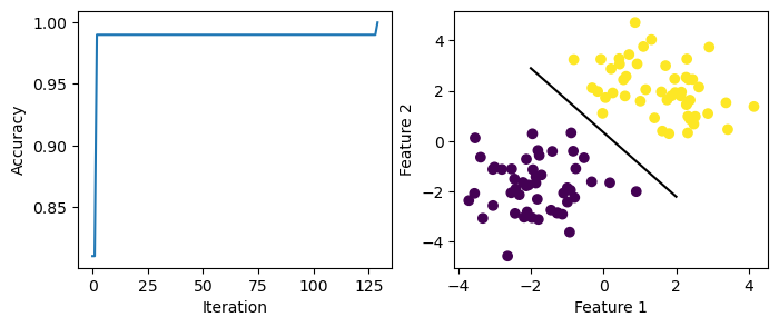

Here, the data is linearly separable. The accuracy is able to reach 1.0 after 125+ iterations. The perceptron line generated is able to separate data with labels -1 and 1.

Non-linearly-separable data

# generate random data
X, y = make_blobs(n_samples = 100, n_features = p_features - 1, centers = [(-1.7, -1.7), (1.7, 1.7)])

# fit perceptron to data
p2 = Perceptron()
p2.fit(X, y, max_steps = 1000)

# visualizations
fig, (ax1, ax2) = plt.subplots(1, 2, figsize = (8, 3)) 

# visualize accuracy history
ax1.plot(p2.history)
ax1.set(xlabel = "Iteration",
ylabel = "Accuracy")

# visualize data points and perceptron line
def draw_line(w, x_min, x_max):
  x = np.linspace(x_min, x_max, 101)
  y = -(w[0]*x + w[2])/w[1]
  plt.plot(x, y, color = "black")

ax2.set(xlabel = "Feature 1",
ylabel = "Feature 2")

ax2 = plt.scatter(X[:,0], X[:,1], c = y)
ax2 = draw_line(p2.w, -2, 2)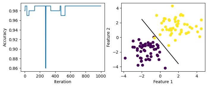

Here, the data is not linearly separable as there are overlapping points. The accuracy fails to reach 1.0 after 1000 steps. The perceptron line does not perfectly separate the two groups of data.

More than 2 features

Here I generate random data with 6 features and feed it to the perceptron algorithm.

# change the number of features
p_features = 7

# generate random data
X, y = make_blobs(n_samples = 100, n_features = p_features - 1, centers = [(-1.7, -1.7), (1.7, 1.7)])

# fit perceptron to data
p3 = Perceptron()
p3.fit(X, y, max_steps = 1000)

# visualize accuracy history
fig = plt.plot(p3.history)
xlab = plt.xlabel("Iteration")
ylab = plt.ylabel("Accuracy")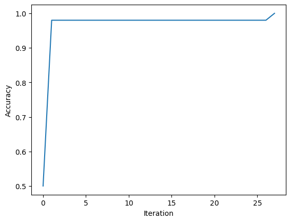

Since the accuracy has reached 1.0, the data should be linearly separable.

Runtime complexity

The runtime complexity of a single iteration of the perceptron update should be \(O(p)\). It would depend on the number of features but not the number of data points.